Usage
This section gives a small tutorial of the core functions of GopPy. A basic familiarity with Gaussian processes is assumed. Otherwise you might want to take a look at [1] first (there is also a free online version).
Creating and Fitting Gaussian Process
Let us first create some toy data from a cosine:
import numpy as np

n = 15
x = np.atleast_2d(2 * np.random.rand(n)).T
y = np.cos(x) + 0.1 * np.random.randn(n, 1)
The orientation of data matrices used by GopPy is samples (rows) times dimensions (columns). Here we use one-dimensional input and output spaces. Hence, both arrays have 15 rows and 1 column. This is the same way scikit-learn handles data.
Then we create a Gaussian process using a squared exponential kernel with
a length scale of 0.5. We also use a noise variance of 0.1. The process is
fitted to the data using the OnlineGP.fit() method:
from goppy import OnlineGP, SquaredExponentialKernel

gp = OnlineGP(SquaredExponentialKernel(0.5), noise_var=0.1)
gp.fit(x, y)
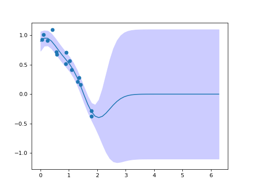
After fitting we can use the Gaussian process to make predictions about the mean function and obtain the associated uncertainty:
import matplotlib.pyplot as plt

test_x = np.linspace(0, 2 * np.pi)
pred = gp.predict(np.atleast_2d(test_x).T, what=("mean", "mse"))
mean = np.squeeze(pred["mean"])  # There is only one output dimension.
mse = pred["mse"]

plt.fill_between(test_x, mean - mse, mean + mse, color=(0.8, 0.8, 1.0))
plt.plot(test_x, pred["mean"])
plt.scatter(x, y)
(Source code, png, hires.png, pdf)

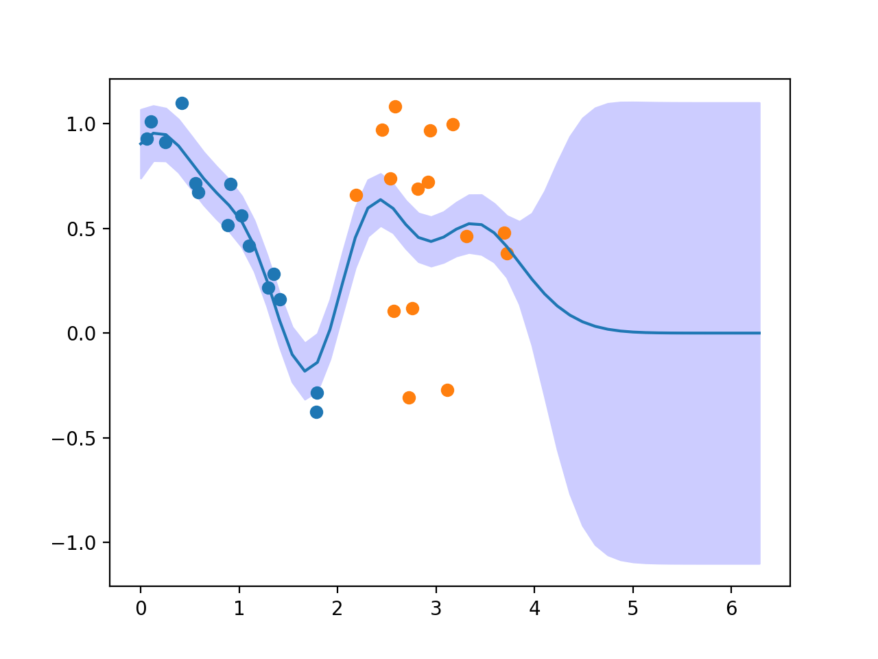
Adding New Data to a Gaussian Process
When further data is obtained, these can be added easily to the Gaussian process
by using the OnlineGP.add() method:
x2 = np.atleast_2d(2 + 2 * np.random.rand(n)).T
y2 = np.cos(x) + 0.1 * np.random.randn(n, 1)

gp.add(x2, y2)

pred = gp.predict(np.atleast_2d(test_x).T, what=("mean", "mse"))
mean = np.squeeze(pred["mean"])  # There is only one output dimension.
mse = pred["mse"]

plt.fill_between(test_x, mean - mse, mean + mse, color=(0.8, 0.8, 1.0))
plt.plot(test_x, pred["mean"])
plt.scatter(x, y)
plt.scatter(x2, y2)
(Source code, png, hires.png, pdf)

If you called the OnlineGP.fit() method multiple times, the process
would be retrained discarding previous data instead of adding new data. You may
also use OnlineGP.add() for the initial training without ever calling
OnlineGP.fit().
Tips
If you know how many samples will be added overall to the Gaussian process, it can be more efficient to pass this number as
expected_sizeto theOnlineGPconstructor on creation.You can also predict first order derivatives. Take a look at the documentation of
OnlineGP.fit().You can also calculate the log likelihood and the derivative of the log likelihood. Take a look at the documentation of
OnlineGP.calc_log_likelihood().